Latent Variable Models & K-Means Clustering
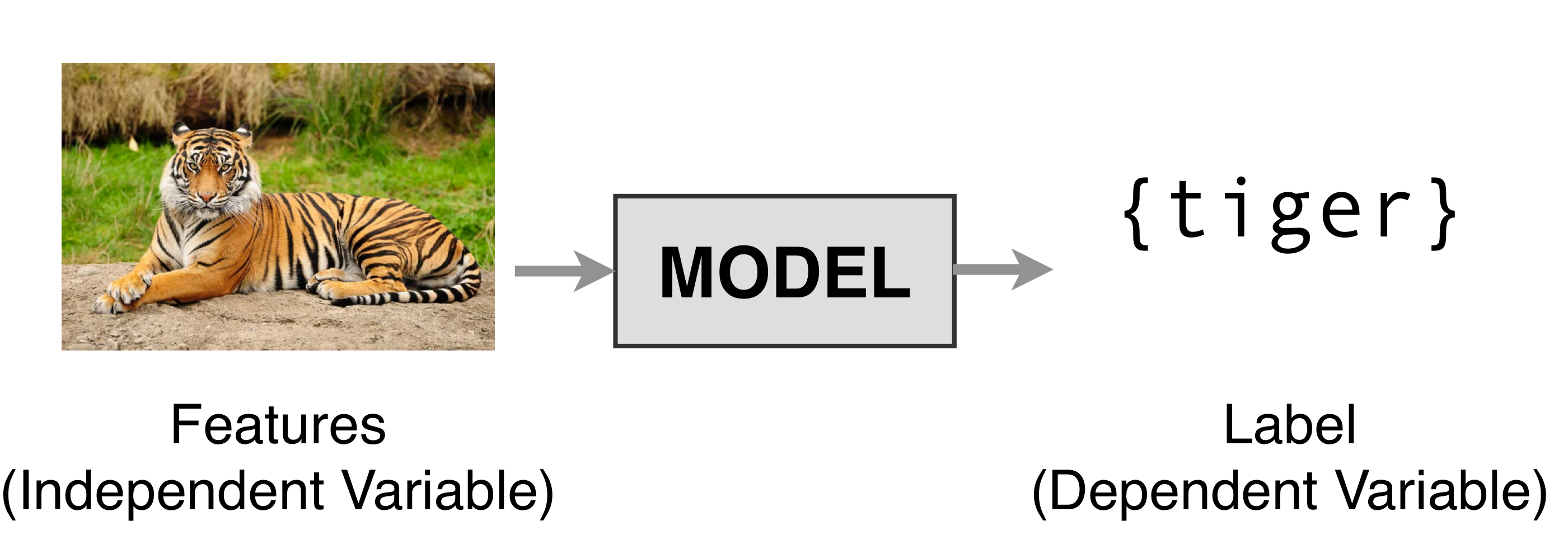
1 Supervised Learning
Here the mission of the model is to learn the relation between the labels and the features.
2 Unsupervised Learning
You do not have labels you only have features.
The mission of the model is to discover latent or hidden structures.
Latent means to be not measurable, to be hidden i.e. thoughts –> words. You can sample words, you have data from the words, but for thoughts you don’t have data available, the variable is hidden
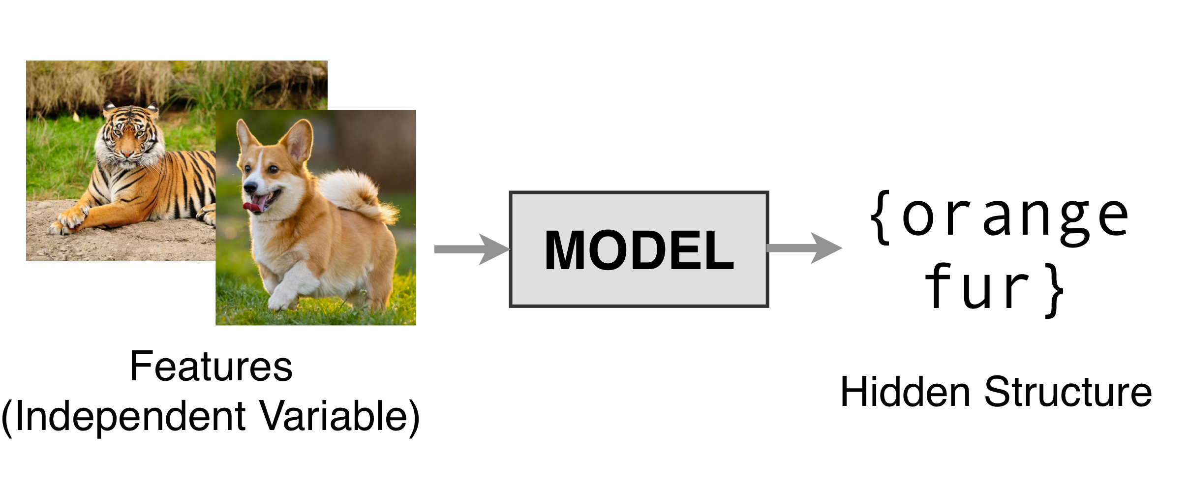
- Unsupervised learning is understanding the data discovering properties to exploit.
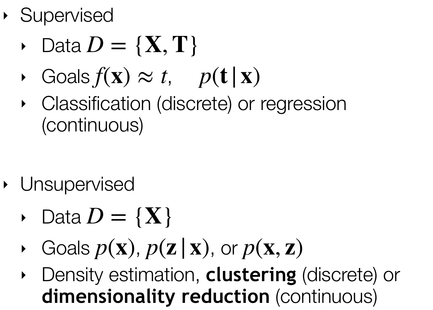
3 Unsupervised vs. Supervised learning
4 Latent variable Models
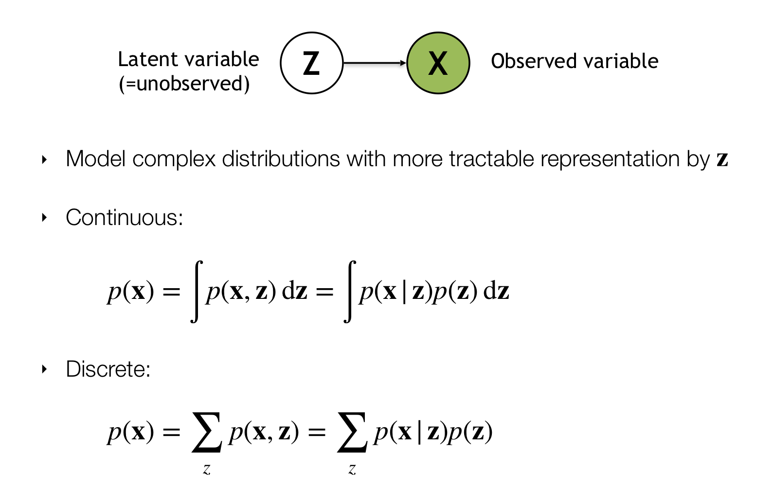
In Unsupervised learning:
You have Latent variable \(Z\) and that generates \(X\).In supervised learning:
For instance in Classification you would have features \(X\) and that generates some label \(y\).
So you could think of Unsupervised learning as we are given our labels and we need to learn the features that generate the label
\(Z\) in the figure above are the labels. We want to get the distriution of the data in the continuous case i.e. by marginalizing over \(z\) to get the probability of the data alone.
5 Examples
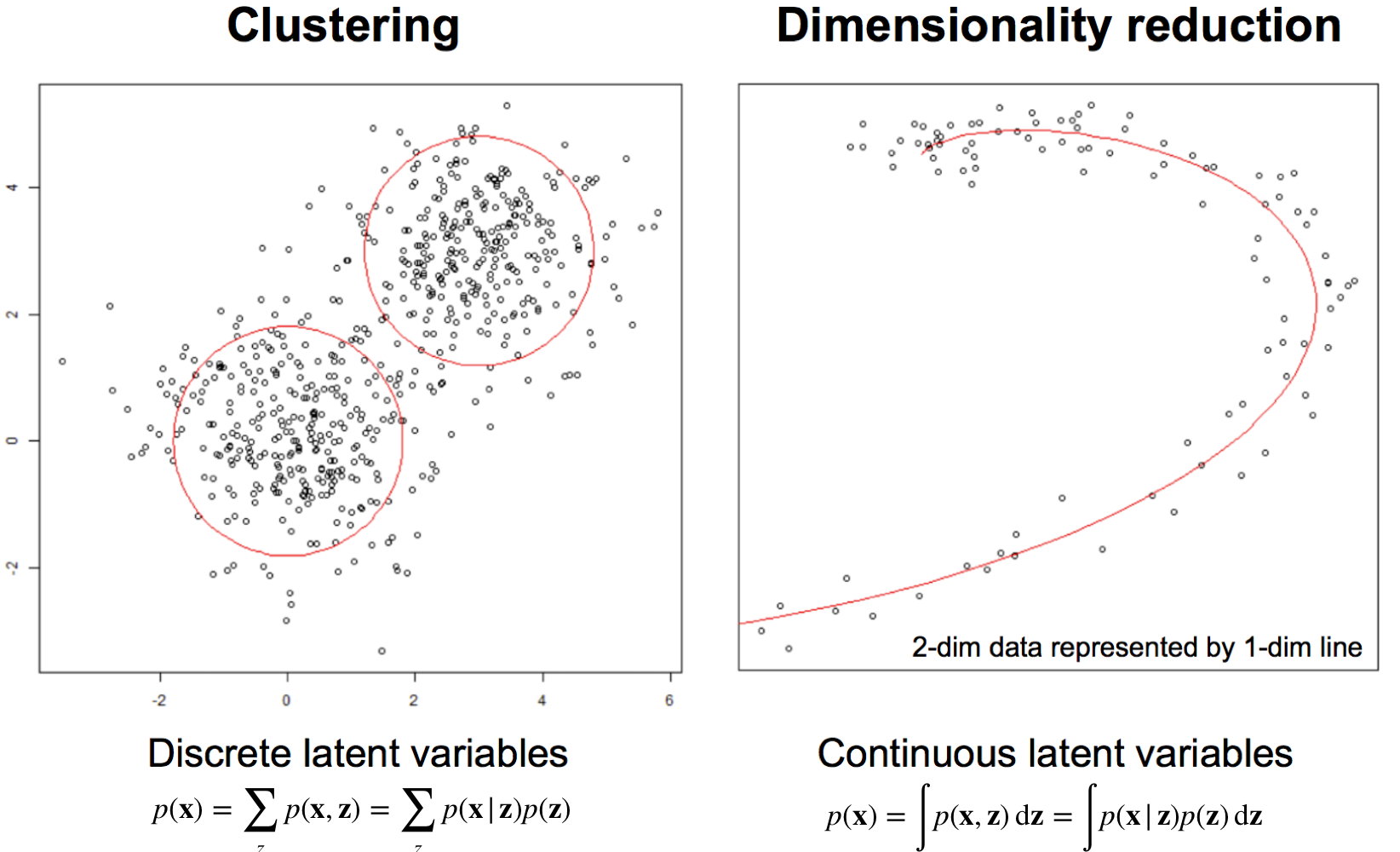
For instance in Clustering we are given scattered plot data and you want to find the hidden groups.
For instance in Dimensionality Reduction you are given a 2-dim data and you wonder whether you can learn a lower representation that could describe my data
6 K-Means Clustering
Goal: Automatically partition unlabeled data into groups of similar data points.
- Useful for:
- Automatically organizing data.
- Understanding hidden structure in data.
- Preprocessing for downstream analysis.
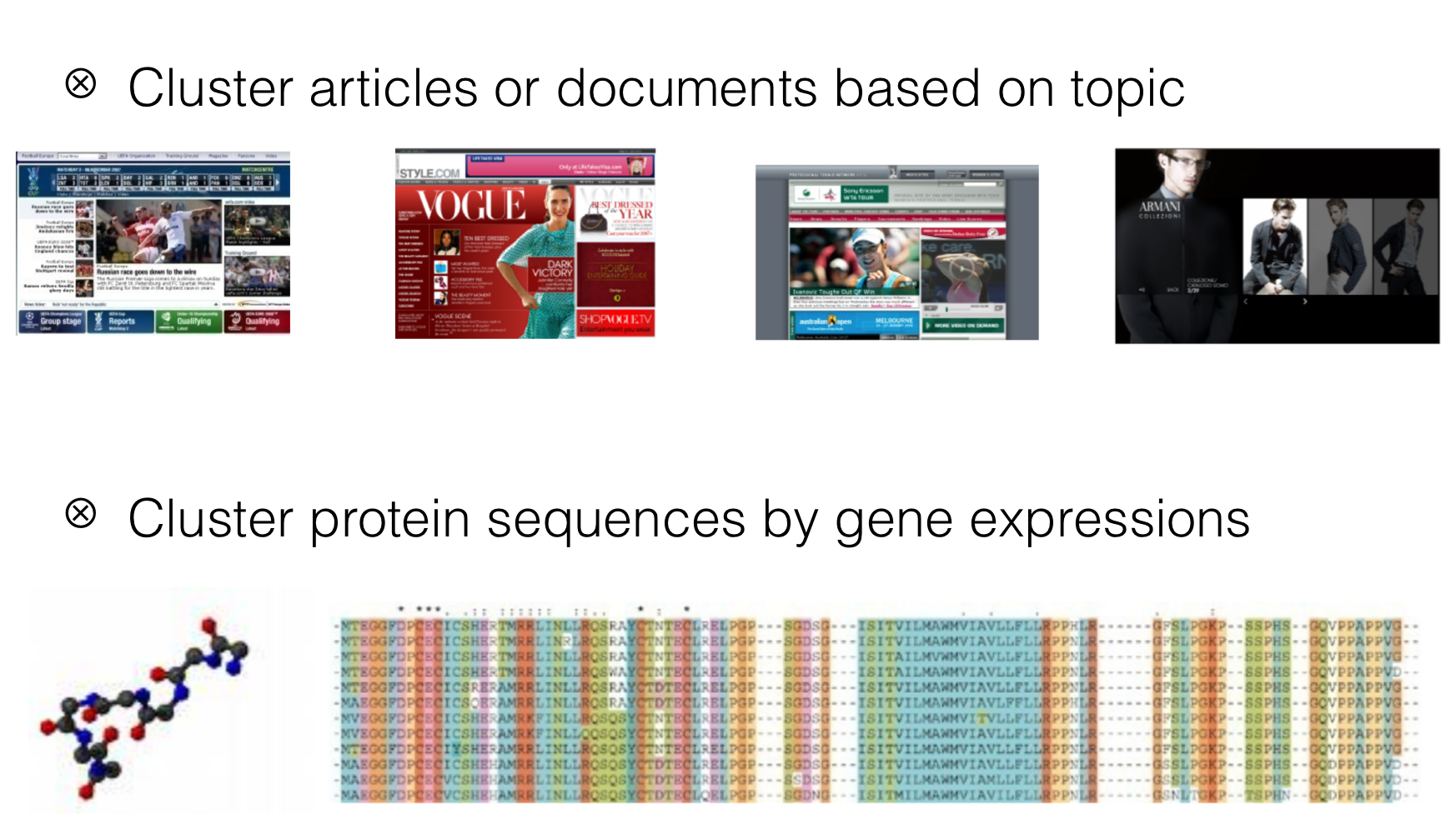
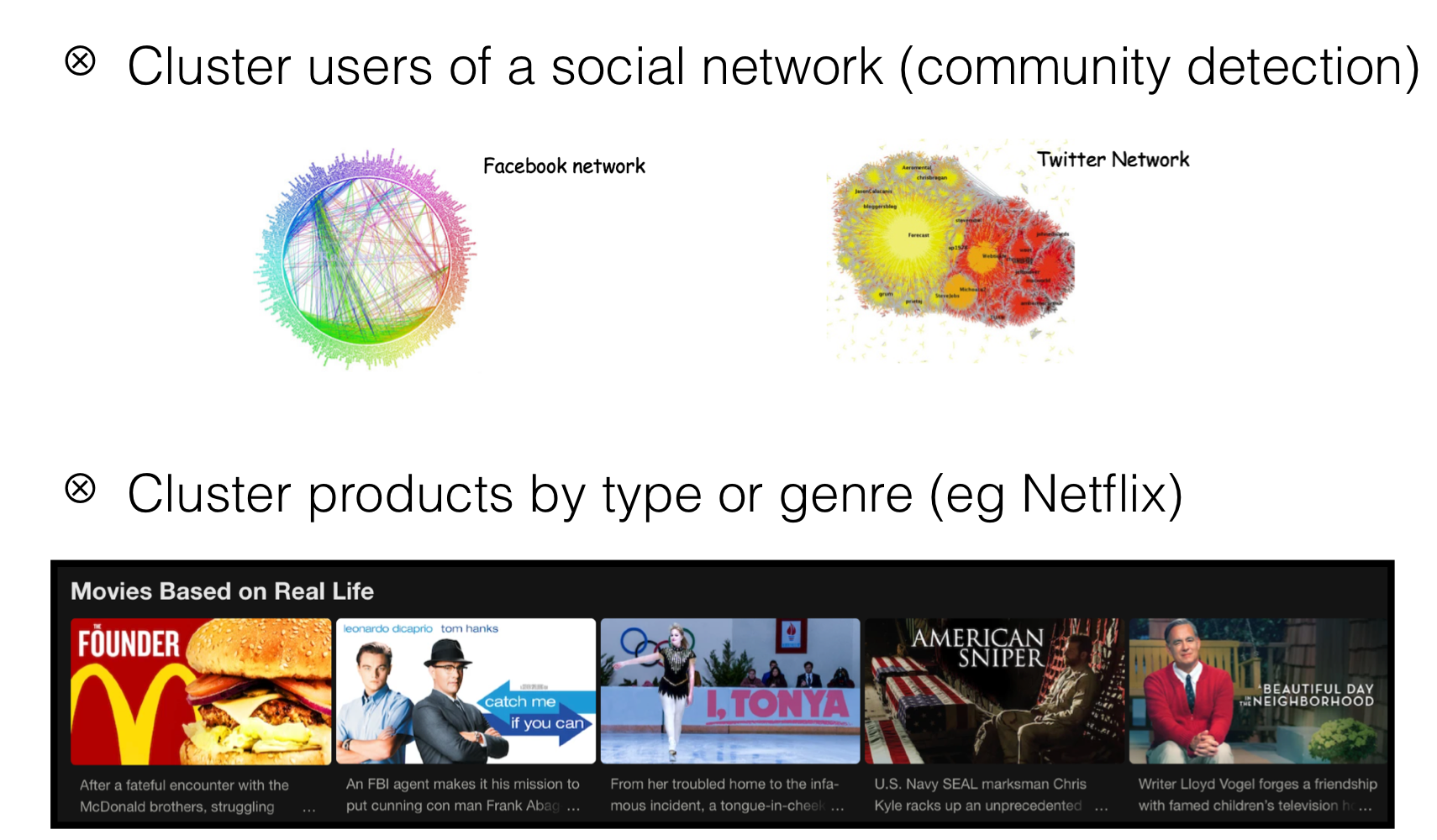
7 Applications
8 Clustering with K-means
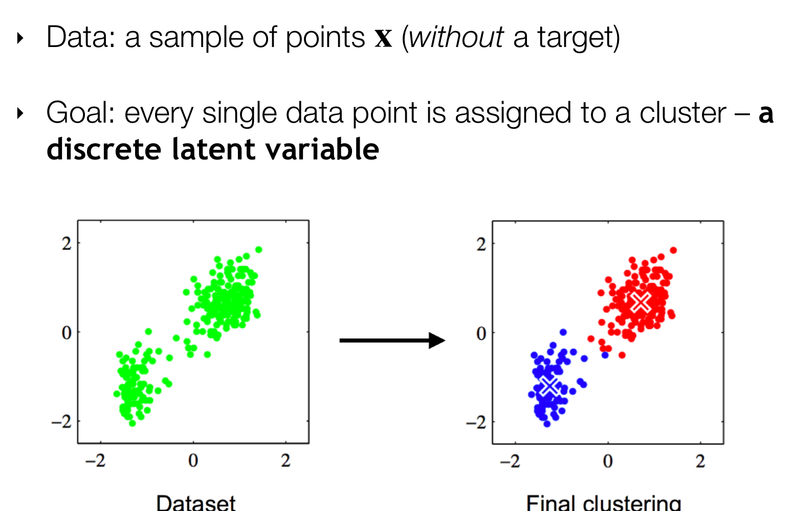
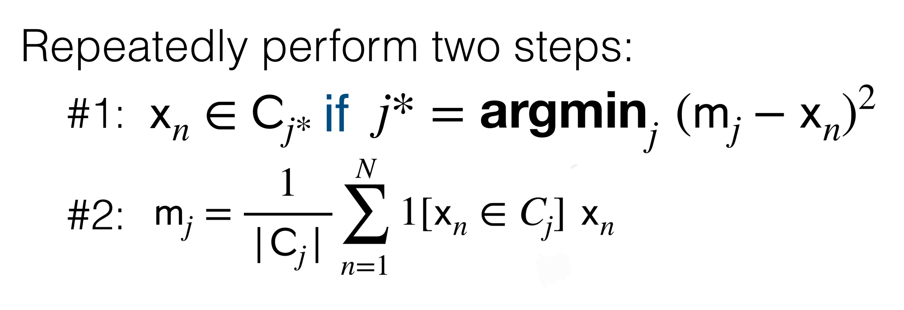
Goal: minimize distance between data points and \(k\) cluster representations
9 K-means
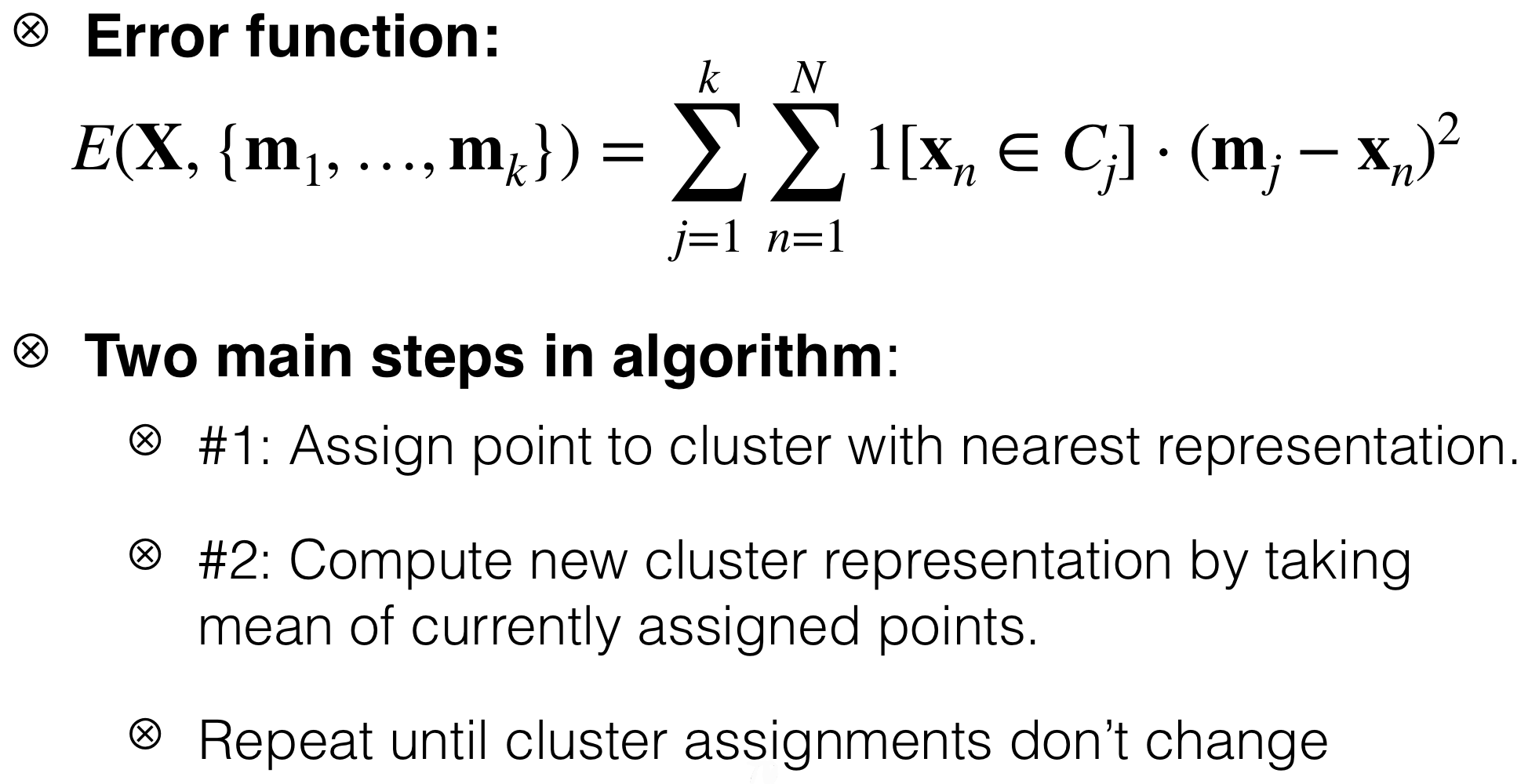
- You need to set \(K\) the number of clusters ahead of time
- The mean \(m_j\) per ach cluster
- The cluster that corresponds \(C_j\)
- You only compute the \(x_n\) that belongs to that cluster \(C_j\) so that we do not compute for all data points
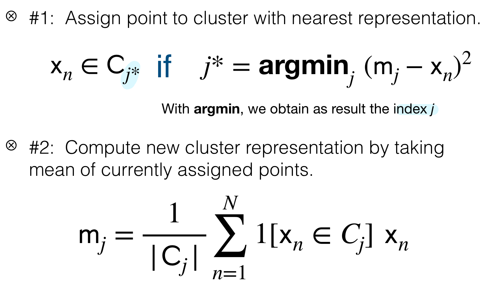
- \(|C_j|\) is the number of datapoints assigned to that cluster \(j\)
10 K-Means Clustering Example
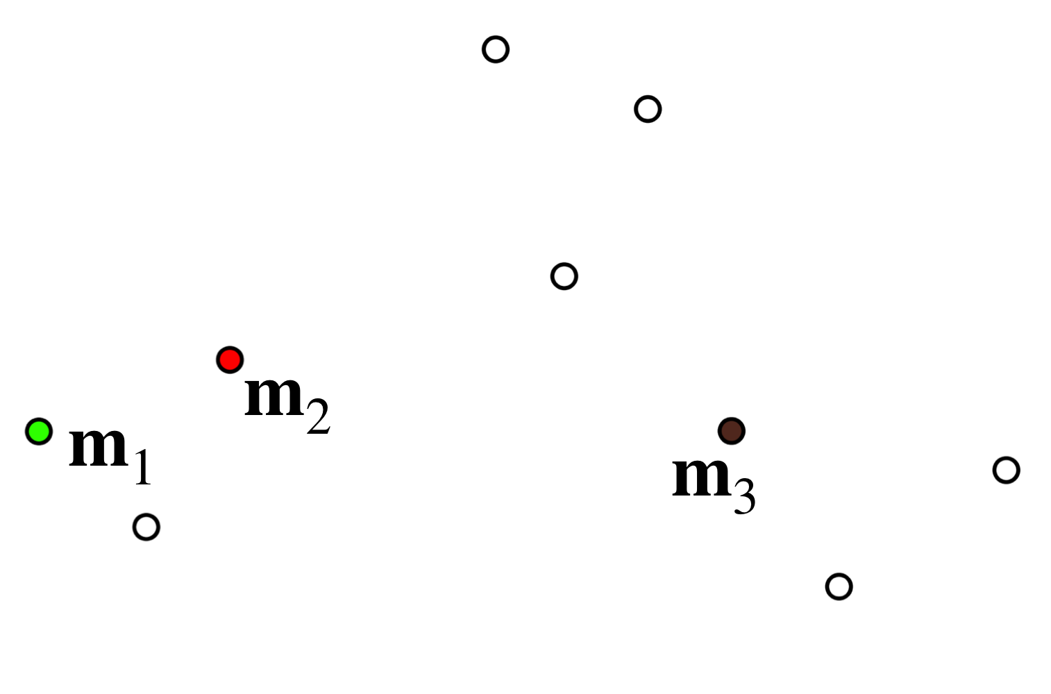
0. Randomly initialize \(k=3\) means to data points. (That means we will end up with \(3\) Clusters)
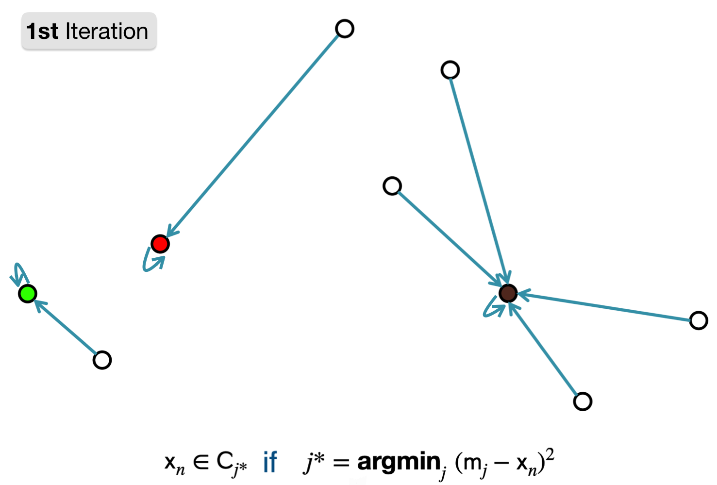
1. Assign point to cluster with nearest representation.
2. Compute new cluster representation by taking mean of currently assigned points.
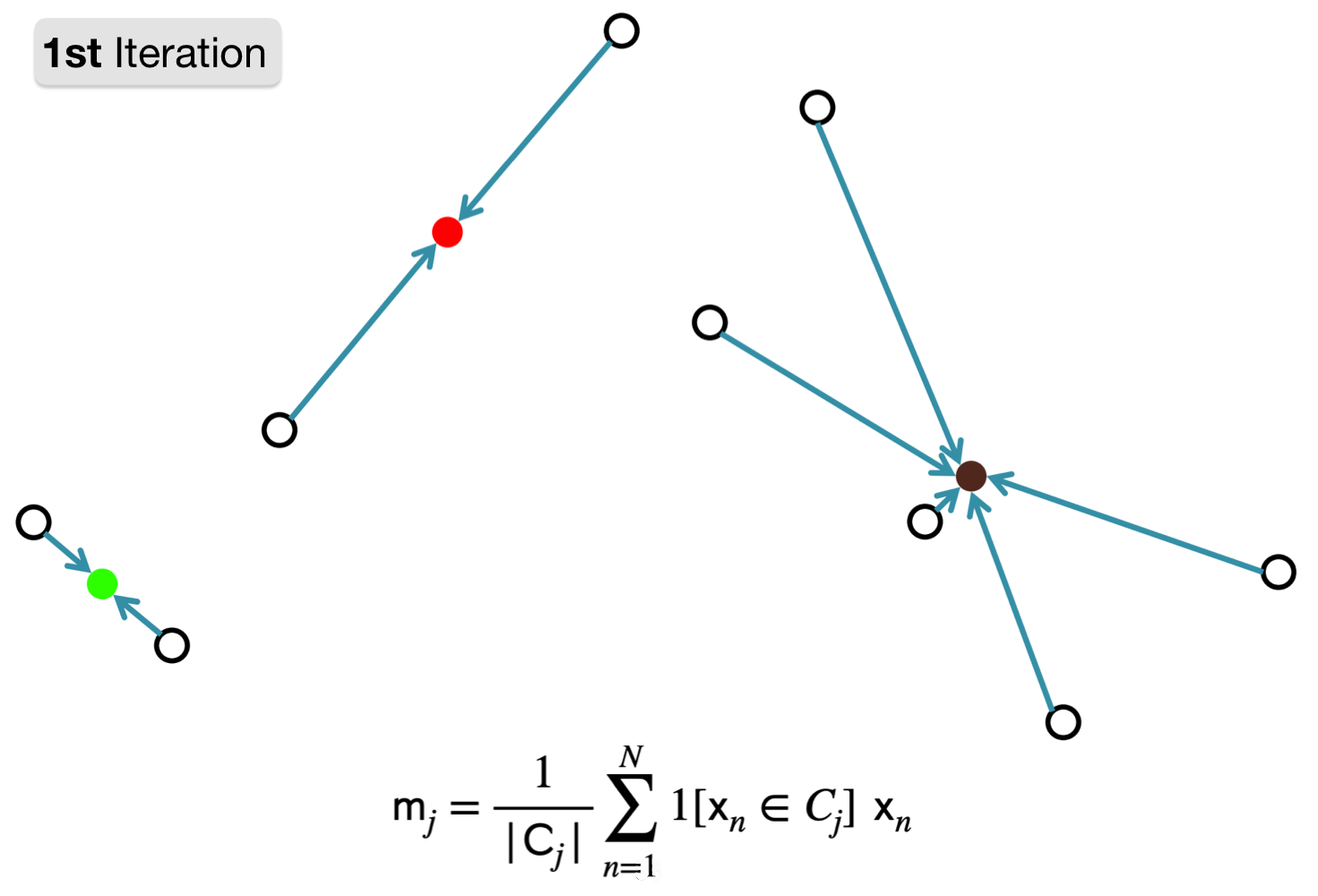
The coloured points you see above are the new computed means. They are NOT data points they are just the locations where the mean should be.
Repeat: Step 1 -> 2
1. Assign point to cluster with nearest representation.
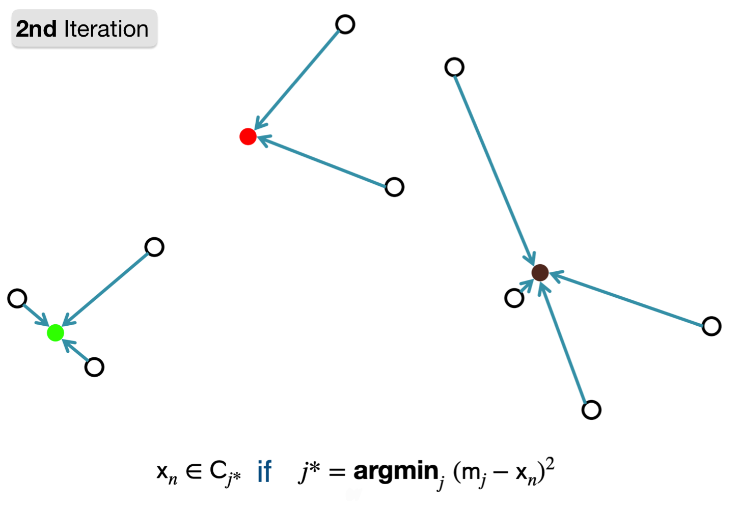
2. Compute new cluster representation by taking mean of currently assigned points.
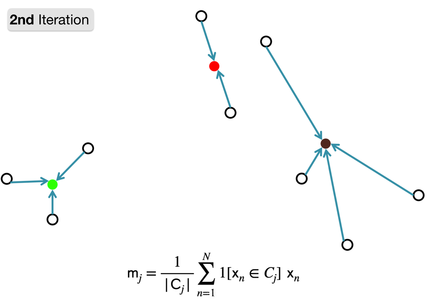
Repeat: Step 1 -> 2
1. Assign point to cluster with nearest representation.
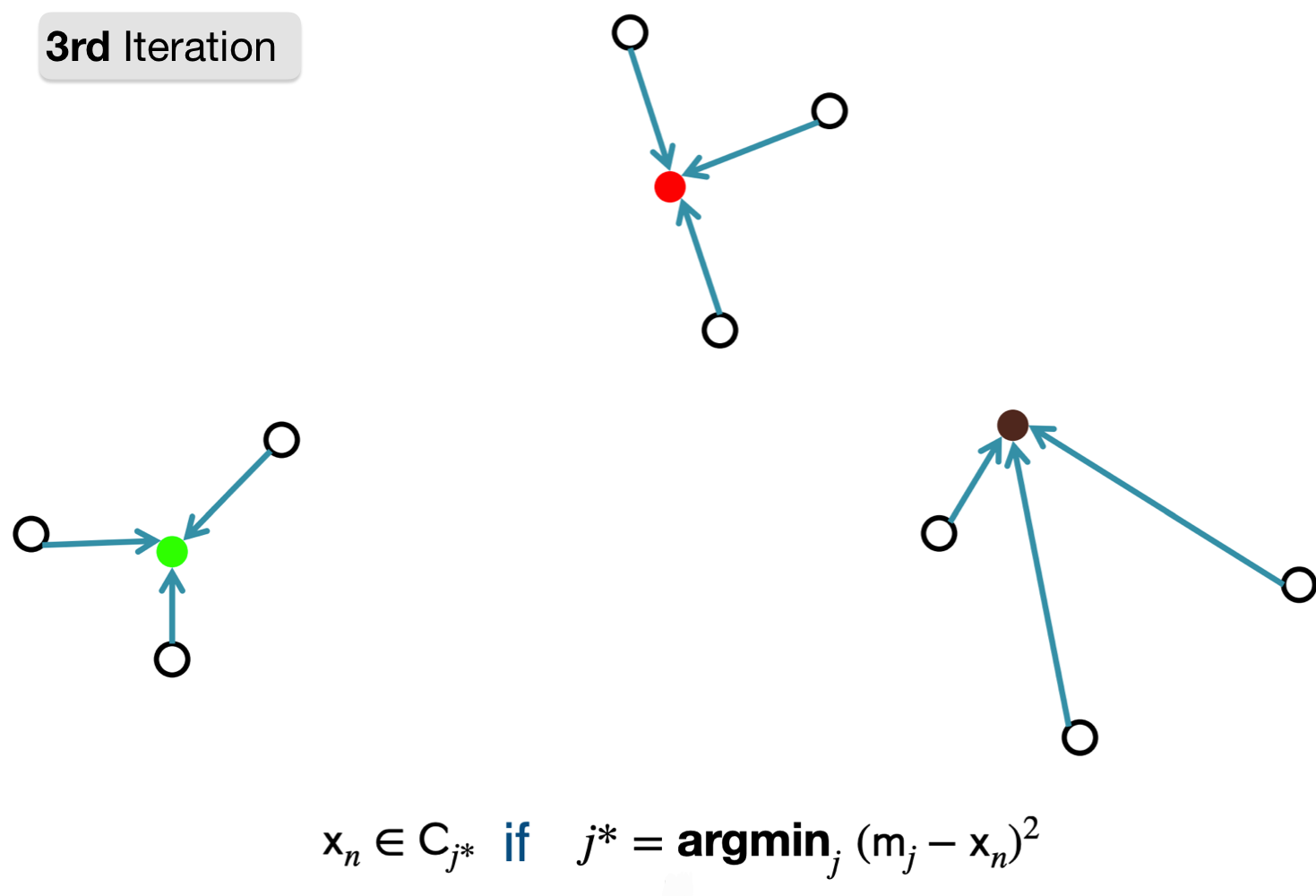
2. Compute new cluster representation by taking mean of currently assigned points.
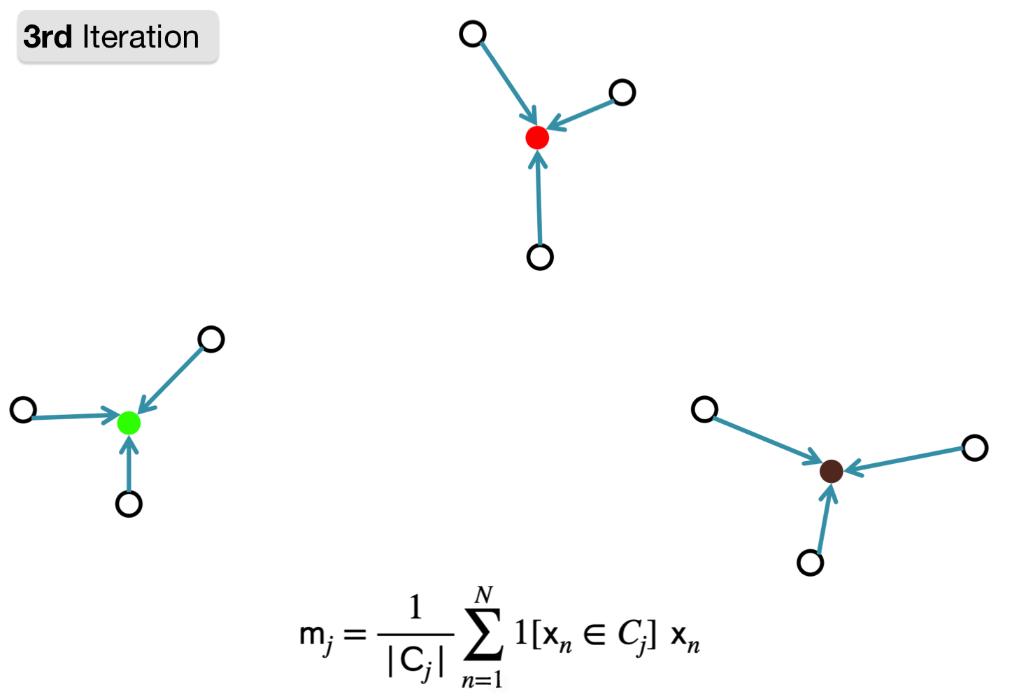
Converging
1. Assign point to cluster with nearest representation.

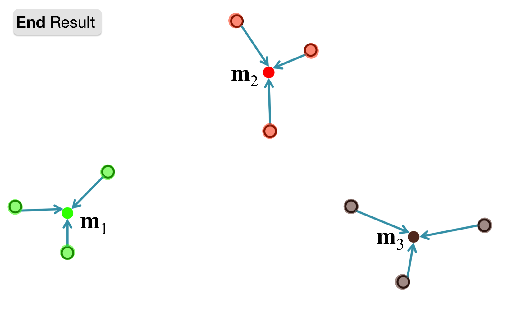
Note: The algorithm has converged: the cluster assignments do not change. So stop here
Final means and cluster assignments
11 K-Means Clustering Pipeline
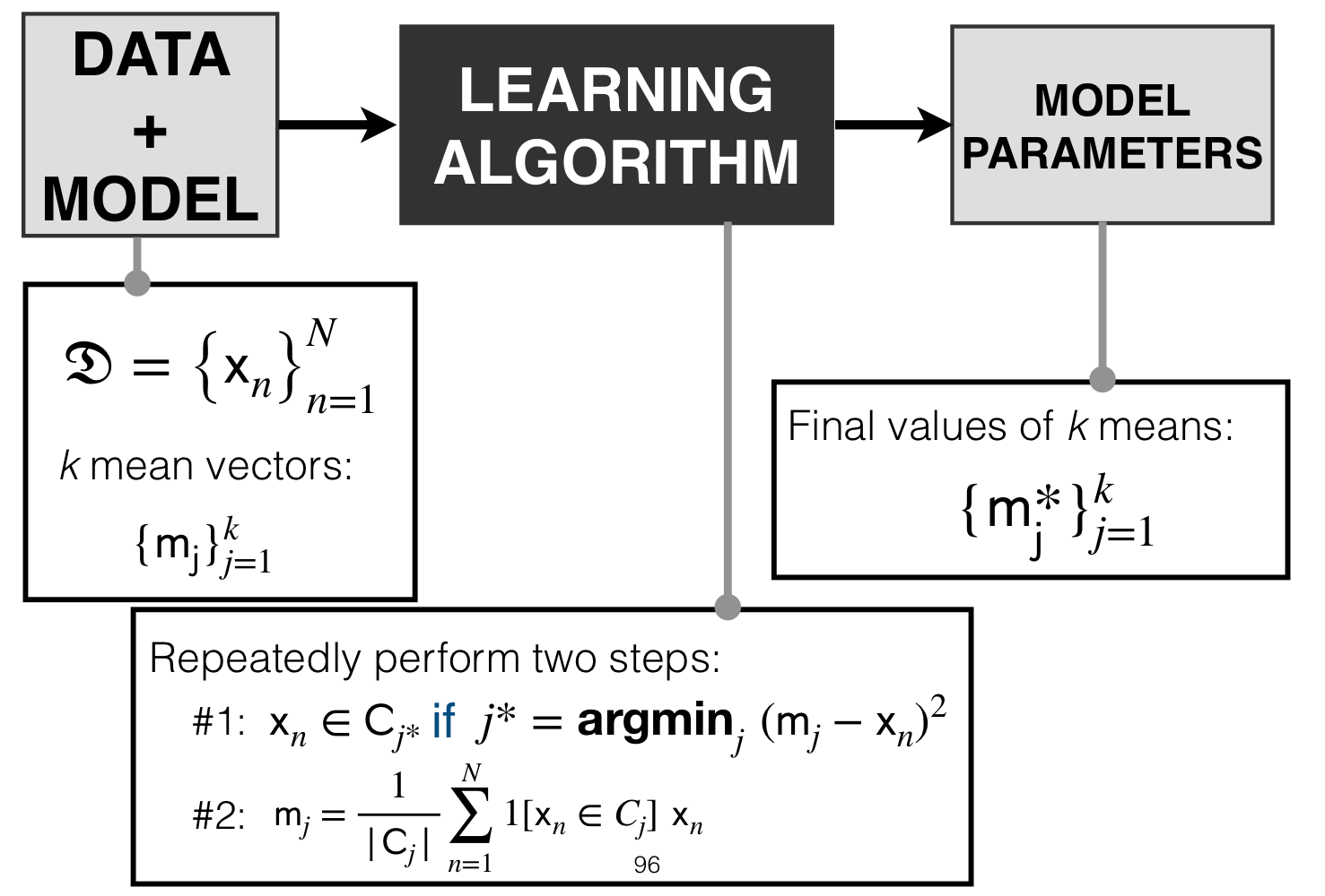
Our model is represented by our \(k\) mean vectors: \(\{{m_j\}}_{j=1}^{k}\)
12 K-Means: Optimization
- The number of iterations to get the same error is lower in the second run
- The cost in the same iteration number is higuer in the first iteration
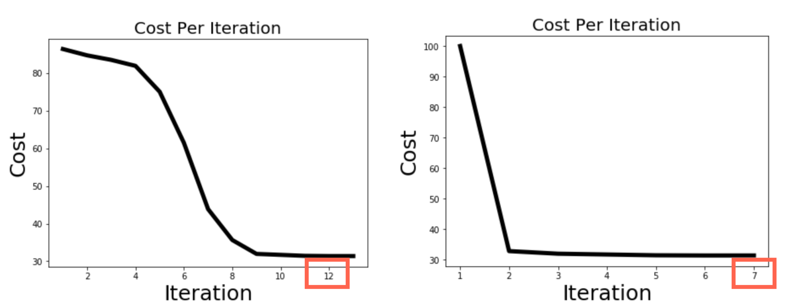
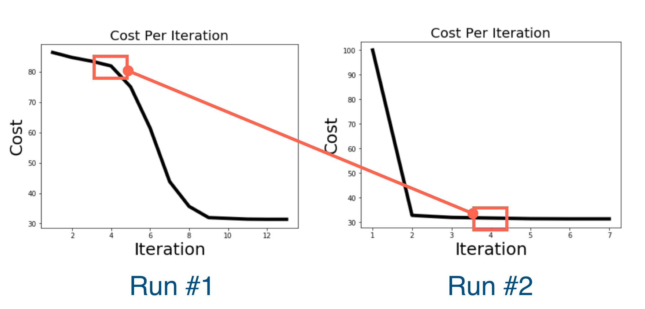
Algorithm guaranteed to decrease error at each iteration, but not guaranteed to obtain Global Optimum.
In between:
- In Linear Regression you can find the global minimum
- In Neural Networks we cannot never find the global optima, we need to adjust our steep size
- In K-means you guarantee to reduce error but not guaranteed that if you keep decreasing you will find global minimum.
For the last reason above (the not guaranteeing thing people in practice re-run algorithm multiple times (and take solution with lowest cost, for instance)
13 K-Means: Overfitting
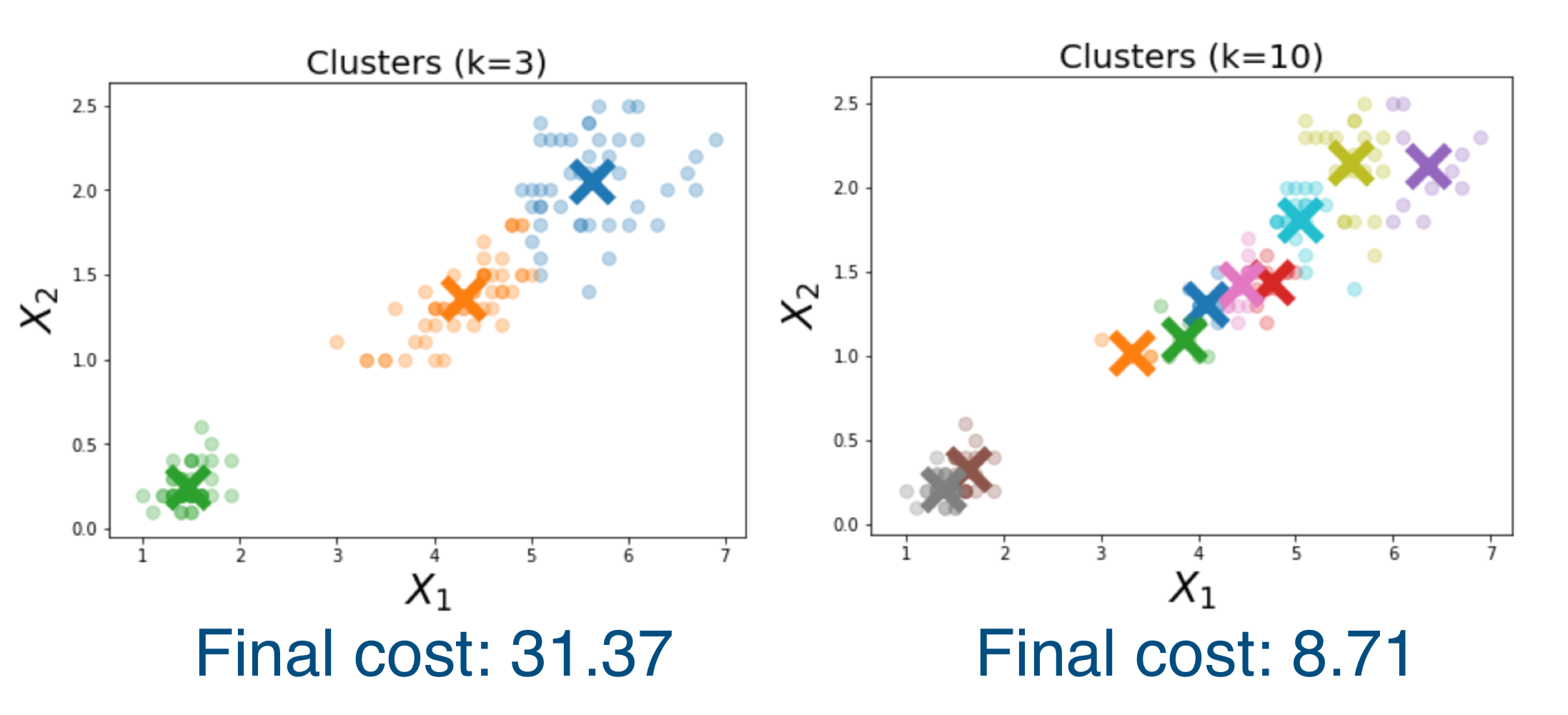
The more clusters we have, the better the chance that a cluster mean will be near held-out data, thus improving the validation error. Thus, looking at validation error alone is not helpful.
So how do we quantify this, because the more clusters then the lower the validation error. How do we choose an appropriate \(k\)-number: Answer with the Elbow method discussed below
14 k-Means: Choosing \(k\)
Method 1
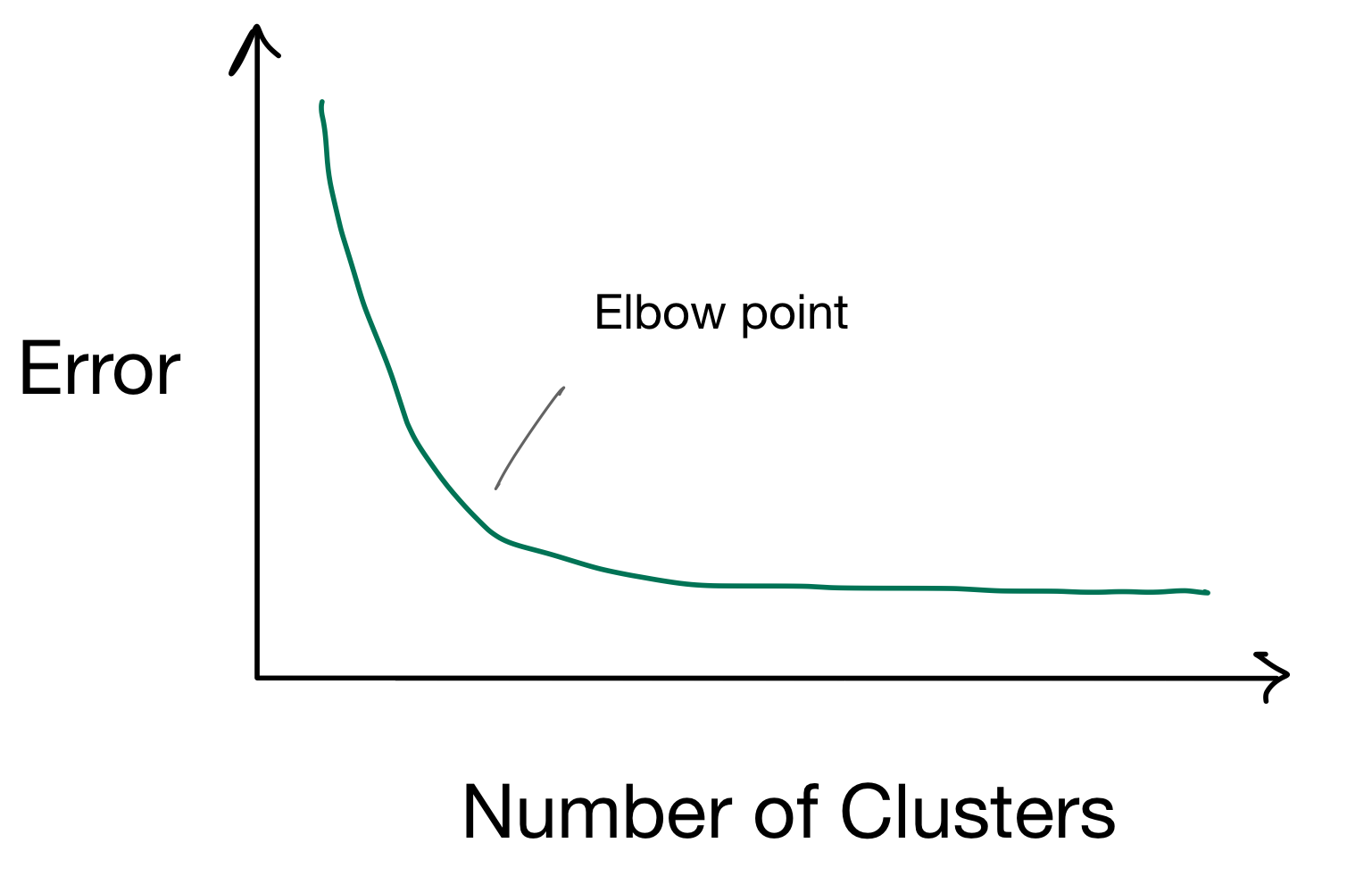
Elbow method: is called like this because think about the error function and your arm. Now we look at the point of hinge where the error loss changes significantly.
For instance in the image below you find your elbow point where adding more cluster does not improve the error.
Method 2
Another method to choose an appropiate \(k\) value is: to have a modified error function that account for the number of clusters:

For instance if I have \(k=1\) then the newly introduced term becomes zero. But if you have more than one cluster it is going to get penalize with a factor \(\lambda\)
Method 3
Here you do external supervision, that means i.e. you have houses clustering by price and size, if you new or wanted to group some houses intentionally then you could stop the \(k\)-size number increasing because you have knowledge domain. Thus you control the granularity.
Method 4

You want the Dunn index to be large, meaning you want in the numerator to be large meaning the minimum distance between cluster representations (so between means) should be large and conversely you want the denominator to be small meaning that you want the maximum distance between points within the cluster to be close to one another (meaning we want to have all point very close to the mean of this cluster)
15 K-Means: Generalizations
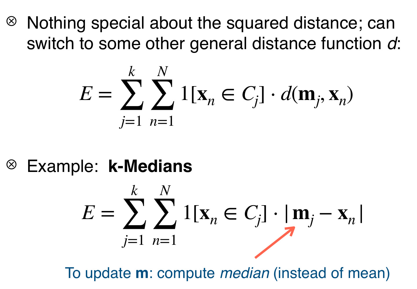
You could also compute the error function \(E\) with other function rather than squarer error, you could for instance use another distance function like Hamming, or medians like below:
16 Improvements for Big Data
- When the data is long then we may take a lot of time to compute one iteration, the solution for this could be to use:
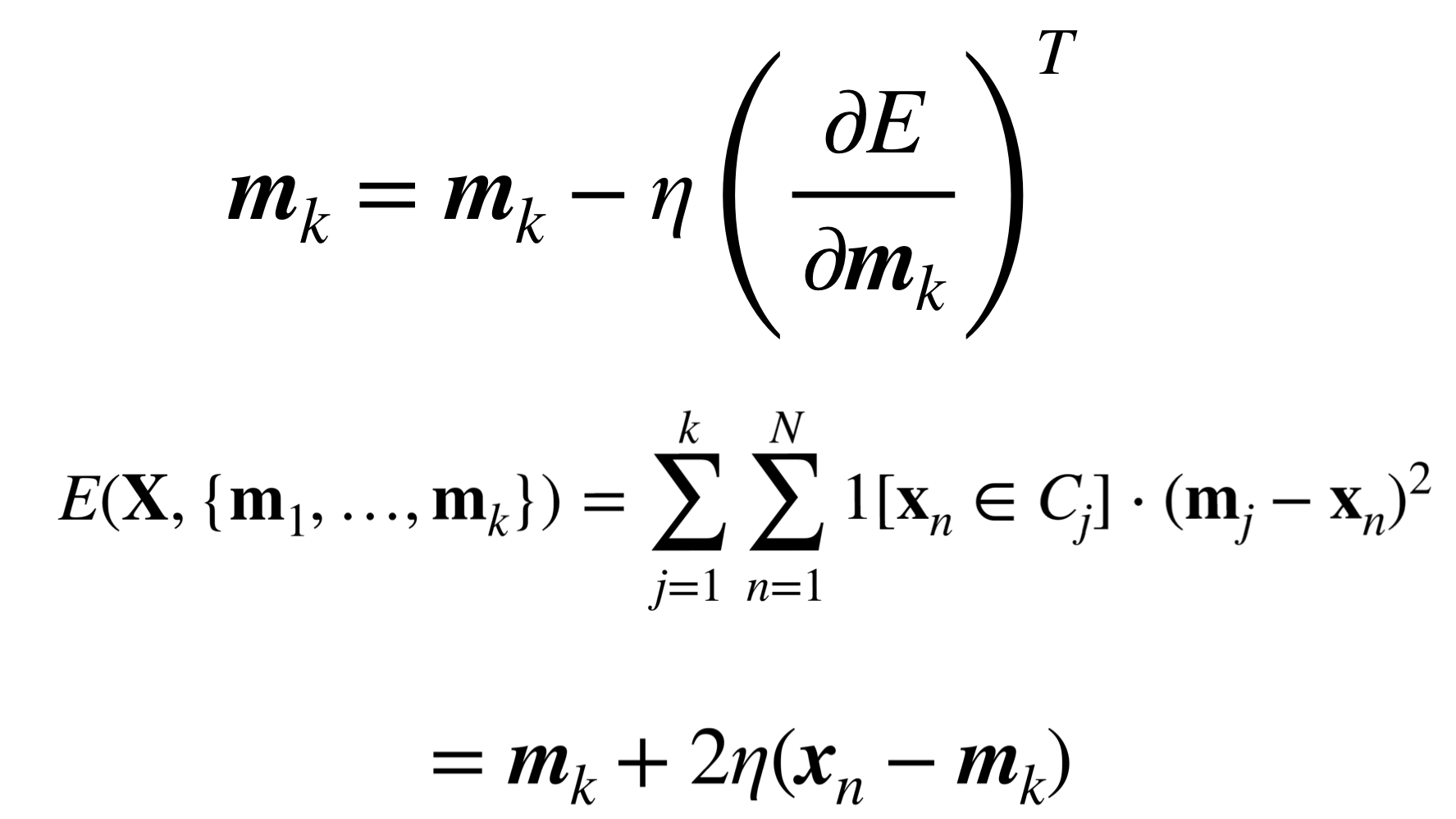
- Stochastic gradient: for each datapoint, update nearest cluster mean”
What this equation is allowing us is to compute the mean not looking at all the data points, again we have the value \(\eta\) which is our learning rate
The mean that we are computing its only nearest to the cluster we compute it
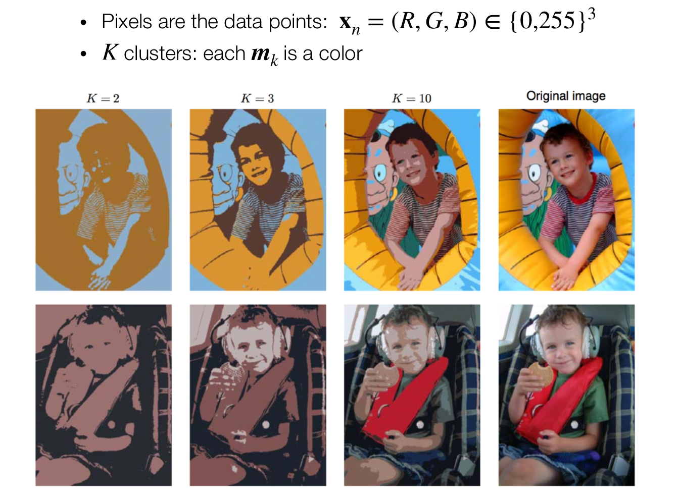
17 Application: image compression
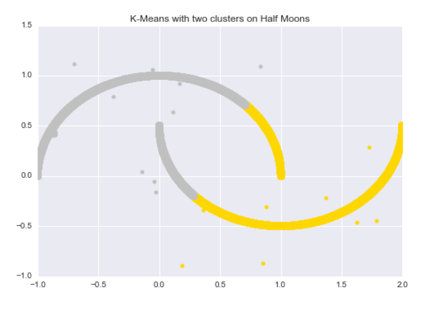
18 Failures of K-Means
This is because of the reliance of square distance, then the points close to the means do not preserve the non-euclidean aspect of this data
Here we should expect to see three clusters: 2 ears and 1 face. The explanation to this is because we cannot modify how th distance will be computed. That means we cannot say that the region of the ears to have a smaller distance, compared to the face’s mean.
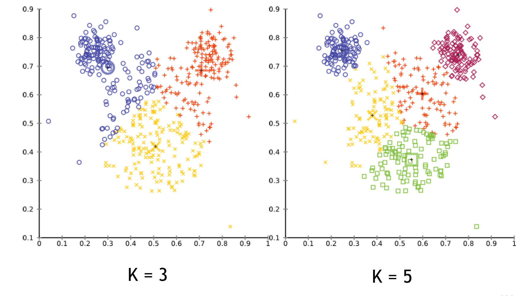
Another way to look at this problems is that, you cannot change the scale of the clusters, every cluster would have more or less the same square distance around its cluster mean. That means that you cannot have tighter distance for the ears and more relaxed notion of distance for the same. They are gonna have same squared distances with equal weight.
19 Pros & Cons of K-Means
- Good:
- Simple to implement
- Fast
- Bad:
- Local minima
- Model only “spherical” clusters that cannot change size
- Sensitive to the features scale
- Number of clusters \(K\) to be chosen in advance
- Cluster assignments are “hard”, not probabilistic => next topic, Gaussian Mixture Model
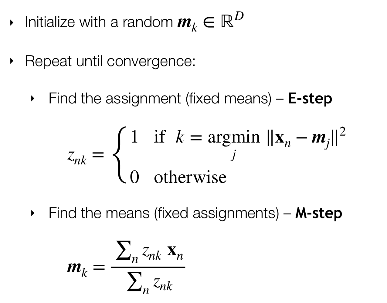
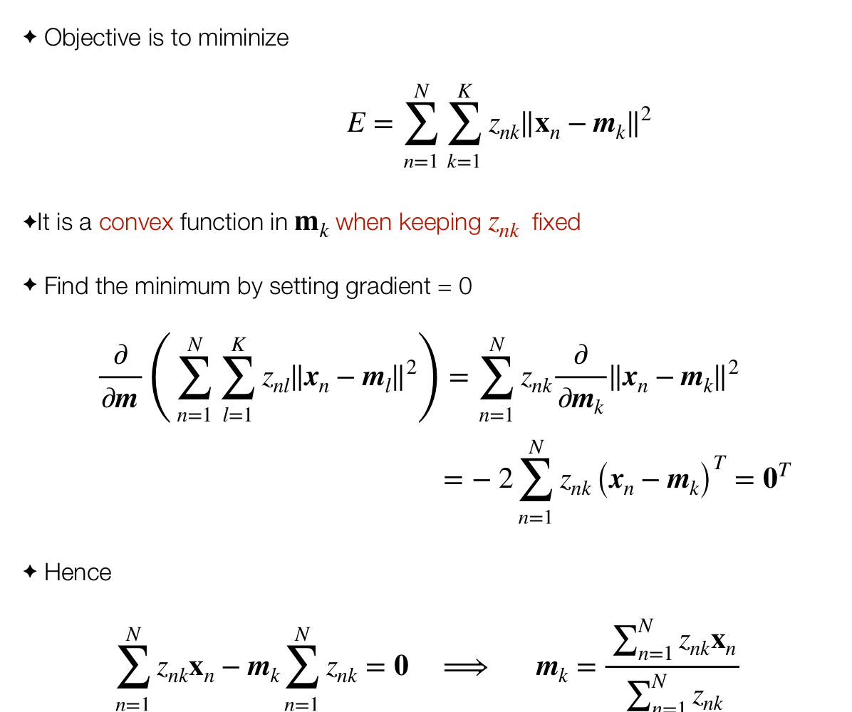
20 Minimize Error (EM Algorithm)
The above algorithm can be formalized in the Expectation Maximization
- The E step computes the assignments
- The M step computes the means
Same as computing:
20.1 Derivation of M-Step
21 Constrained optimization
21.1 Lagrange Constrained Optimization: Example
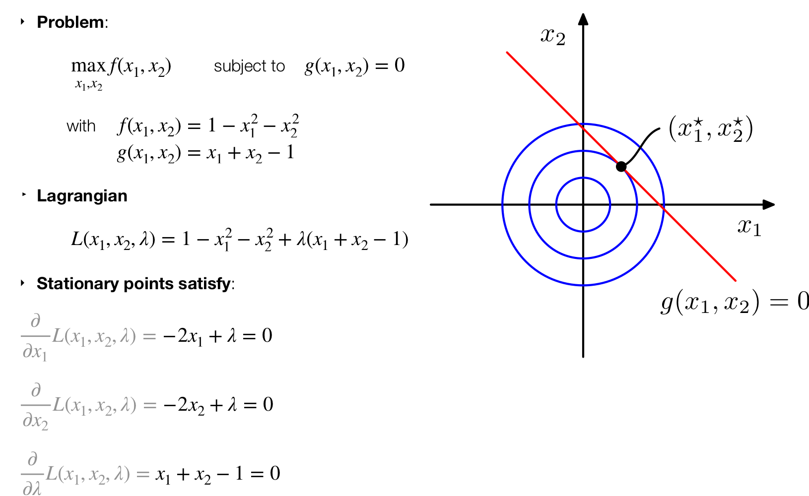
Probabilistic version of k-Means Clustering
In this section we talked about the probabilistic side of k-means
22 Clustering with Gaussian Mixture Model (GMM)
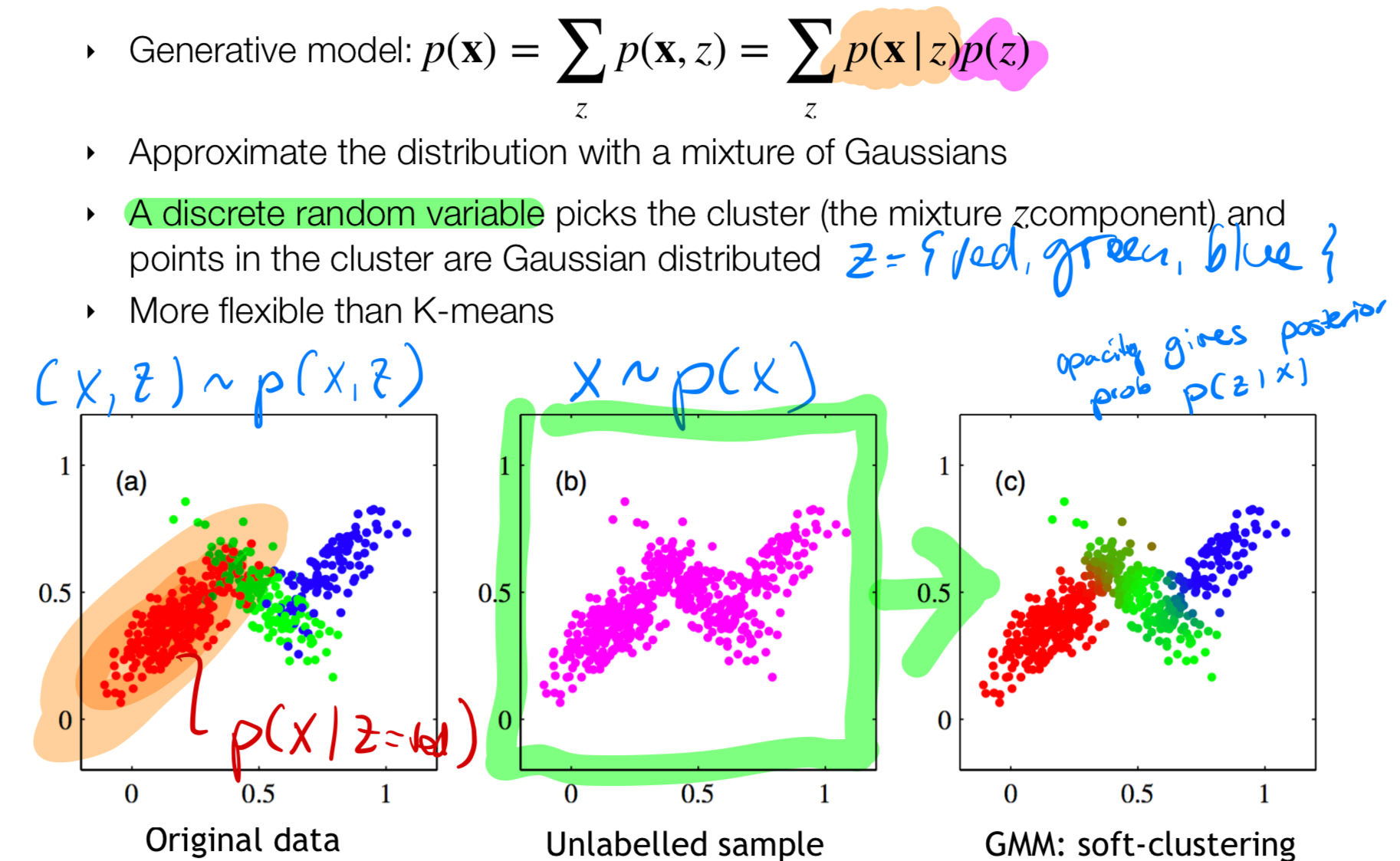
- We assume that the data follows a generative model. Recall what a generative model is:
Approaches that explicitly or implicitly model the distribution of inputs as well as outputs are known as generative models, because by sampling from them it is possible to generate synthetic data points in the input space.
- We also assume that with each observation there is an associated discrete latent variable. Recall what latent variable is:
A latent variable is a variable that is not directly observed is hidden like our thoughs, that is z
For instance: in the image below we see that the purple data, each of these dots is related to a latent variable \(z\), for instance a discrete class \(z\) i.e, that can take on the values {red, green, or blue}. Now these latent variables are hidden is not directly observable, you dont’ know them. Here the latent variable is discrete can take values like: red, green and so on, can also be like the example of the houses, it can be boat houses, studios and so on.
Recap from the upper text. It means that we are no seeing the bottom left graph with the distinctions between classes but we only see the purple dots
- We also assume there is a join distribution \((x,z) \sim p(x,z)\) so in this case in the left plot
Goal: given our unlabelled data \(x \sim p(x)\) (purple dots) you want to go to a cluster ( from our latent variable) assignment. Mathematically you want to be able to compute \(p(z|\textbf{x})\) which is the right bottom graph where you see all datapoints assigned one color. For instance you want to say that a purple dot in the corner belows to class \(z = green\) or another dot that belongs to \(z = blue\). How do we do this? Sol: in a probabilistic way using Multiple Gaussians hence called Gaussian Mixture models.
23 Modelling assumptions
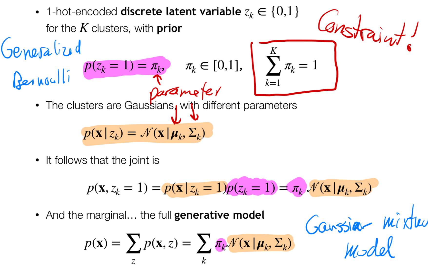
- We model our prior with a Generalized Bernoulli distribution
Categorical Distribution: \[ P(X = x_i) = p_i, \quad \text{for } i = 1, 2, \ldots, K \]
where \(p_i\) is the probability of outcome \(x_i\), and \(\sum_{i=1}^{K} p_i = 1\).
Generalized Bernoulli: \[ P(X = x) = \theta^x (1 - \theta)^{1 - x}, \quad \text{for } x = 0, 1 \]
where \(\theta\) is the probability of \(X = 1\), and \((1 - \theta)\) is the probability of \(X = 0\)
The second part part of our generative model is the latent class or conditional distributions \(p(\textbf{x}|z_k)\) modelled with Gaussians. NOTE this is not the likelihood
- \(p(\textbf{x}|z_k)\): is the probability that if I know the class \(z_k\) then I will observed the data in i.e the red region, see picture above in orange highlighted
The \(\pi_k\), \(\mu_k\), \(\Sigma_k\) are learnable parameters
With the prior and the latent conditional distribution we can compute the joint \(p(\textbf{x},z_k =1)\). That is, we compute the probability for each class
Given this model we can define a \(p(x)\) for the entire data set which is simply the marginalization over \(z\). But this is gonna be a sum of Gaussians, see the equation at bottom of slide. Because of the sum of gaussians we call it Gaussian mixture model
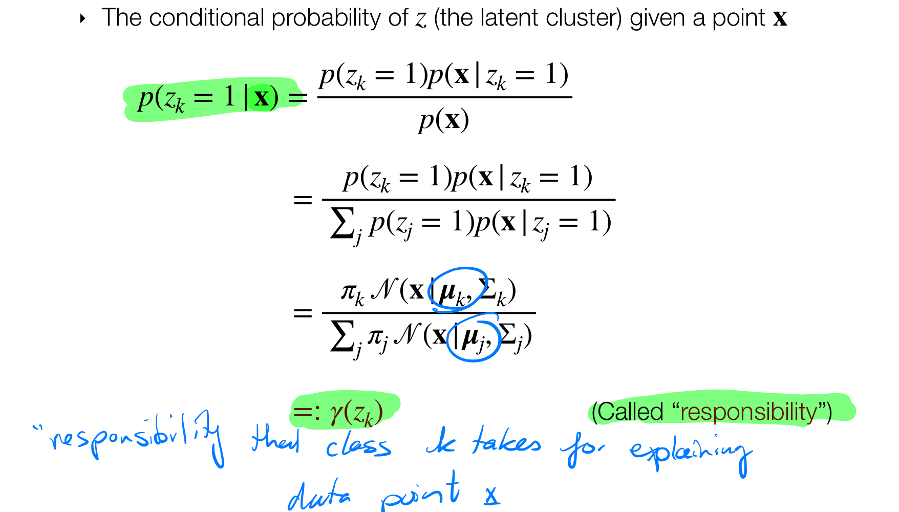
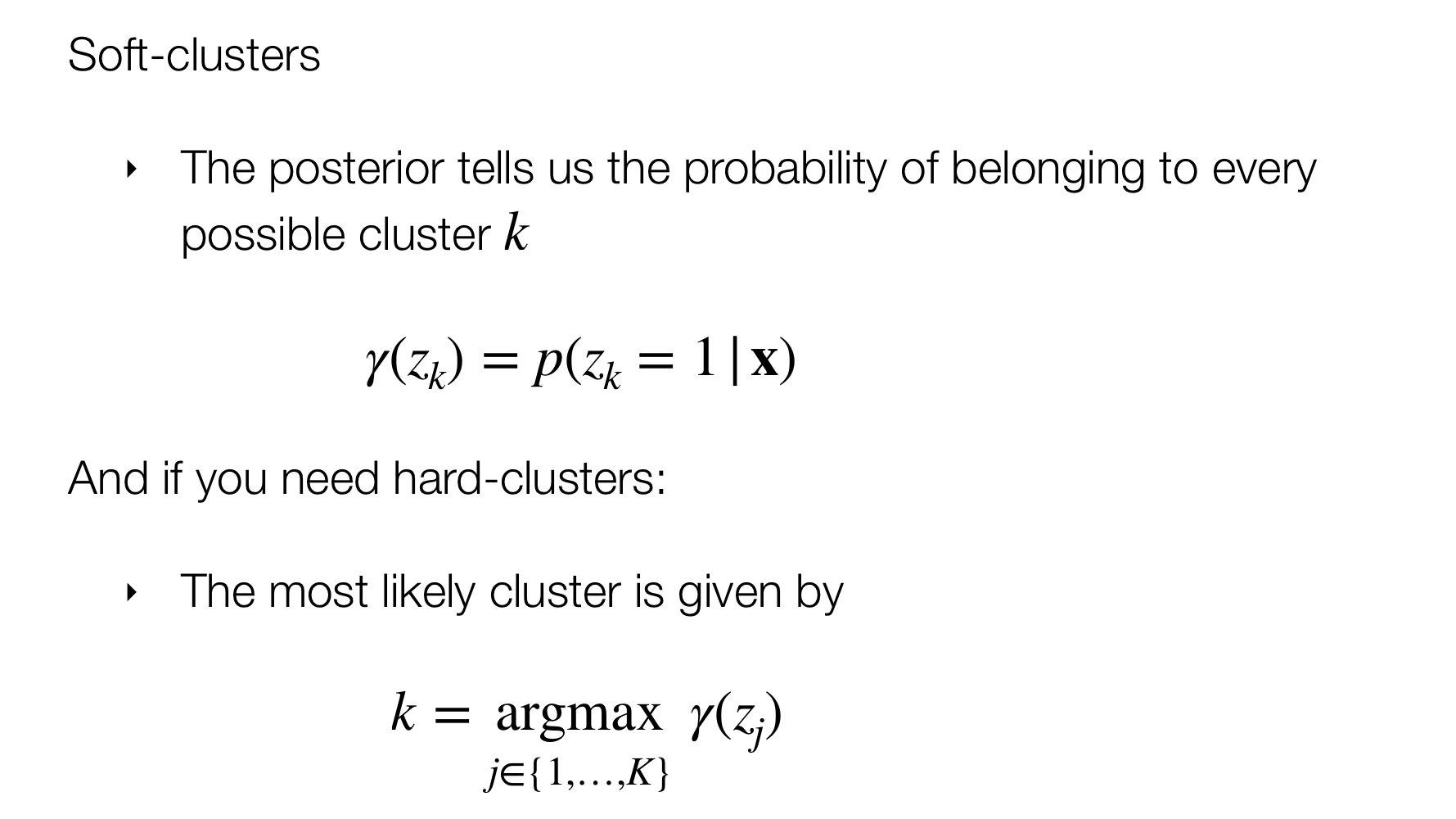
This is how we model \(p(x)\) but now we want to optimize it and since we are working in a probabilistic setting: we can compute the posterior \(p(z_k=1|\textbf{x})\) which we know we can get it with Bayes rule.
- \(p(z_k=1|\textbf{x})\) I have a observation x and we want to know to which class \(z\) it belongs. But this will give a opacity meaning its not totally certain
Recall our goal is to get: \(p(z_k=1|\textbf{x})\). Also recall that in k-means we have a hard assignment of labels. in this case because we are using probabilities then we will end up with soft assignment which means that we will have i.e. one point as green color but also a bit transparent with a red color.
23.1 The Posterior
23.2 The Log-likelihood
- The likelihood can be optimized i,e by taking the log and then derivative with respect to its parameters \(\mu_k\), \(\Sigma_k\)
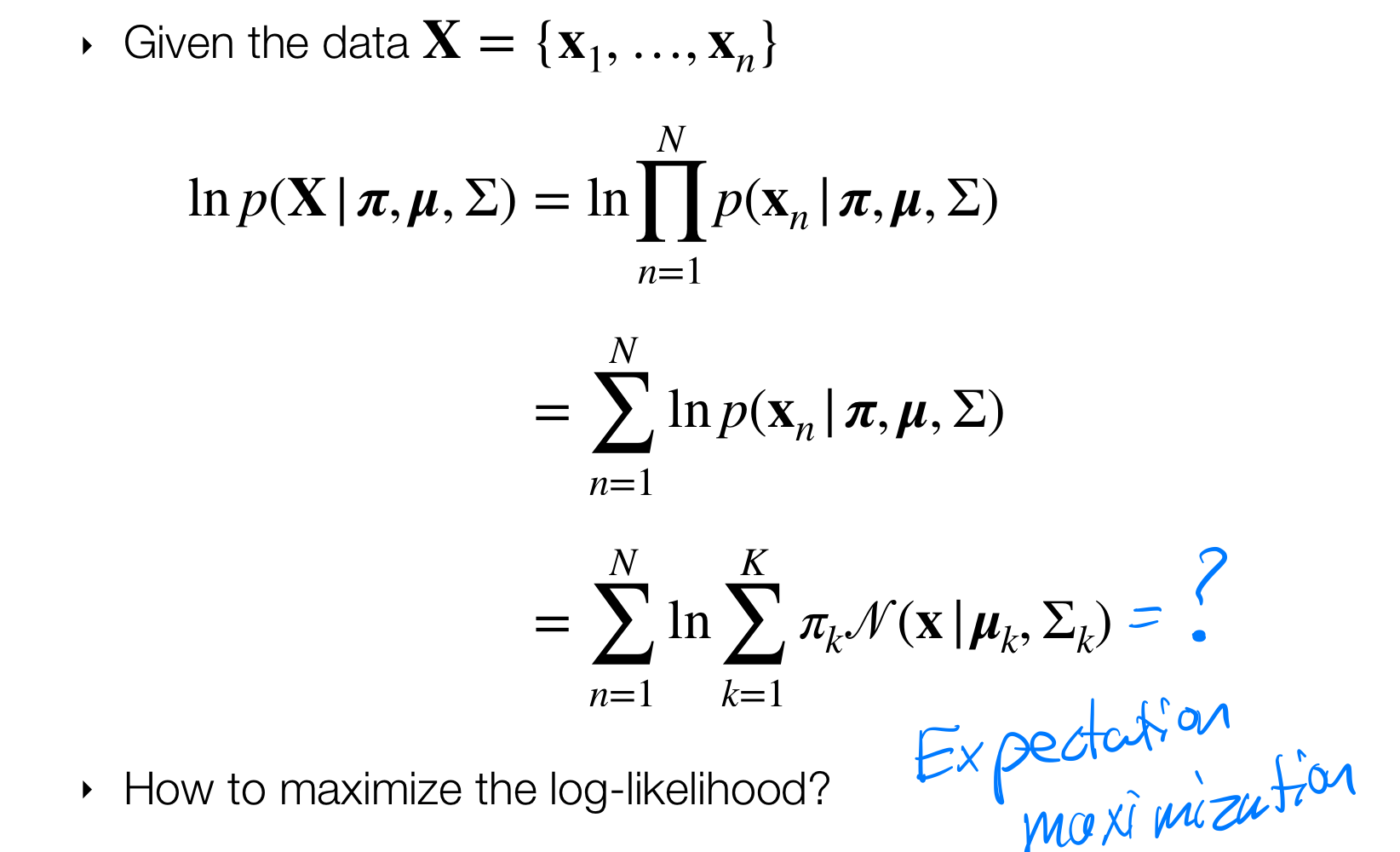
Wait a min, but when you replace the gaussian (which is how we assume to model the data) then because of the sumation over \(\pi_k\) things get matematically and analitically complicated and then we need to resort in another optimization rather just taking the derivative and set it to zero. Thus Expecation Maximization comes into play
Crucial bit why we are taking the log-likelihood as \(p(\text{x})\). See this below:
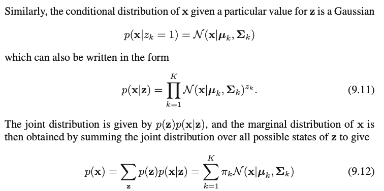
- That is why we compute:
24 Expectation-Maximization algorithm (EM)
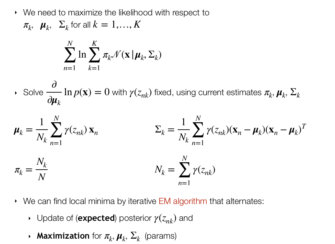
- Here we assume the posteriors \(\gamma(z_k)\) do not depend on the parameters
How to get to teh answers for the parameters?
- With the values for the parameters anc compute the expected posterior
- Maximize for parameters
The cycle repeats
25 Example: GMM
- Here the optimization of the likelihood is called Maximization
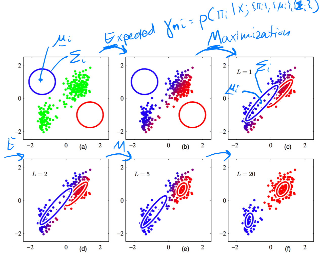
In K-means I only updated the cluster centers whereas here I update all the parameters \(\pi_k\), \(\mu_k\), \(\Sigma_k\)
26 Derivations for EM algorithm
Refer to slides
27 The mouse data again
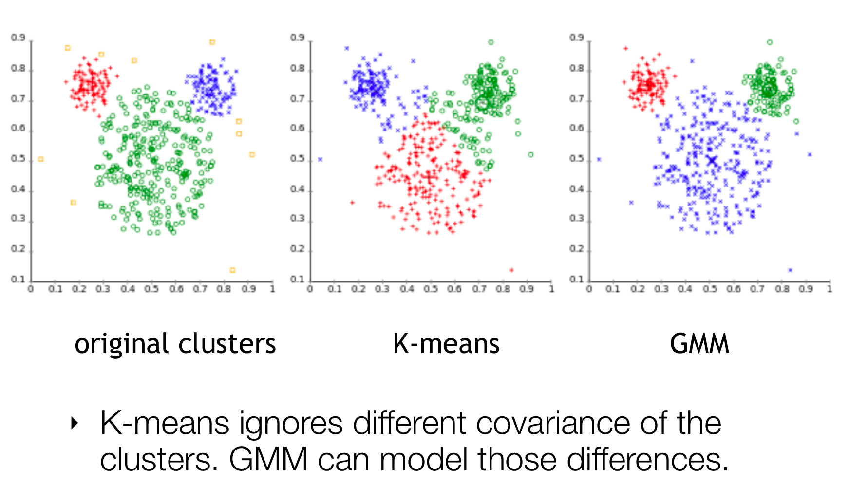
Differences between K-Means and GMM: - K-means can only custer groups of the same size, so same distances from each mean cluster - GMM can compensate for this
28 How do we assign points to cluster?
29 Final remarks
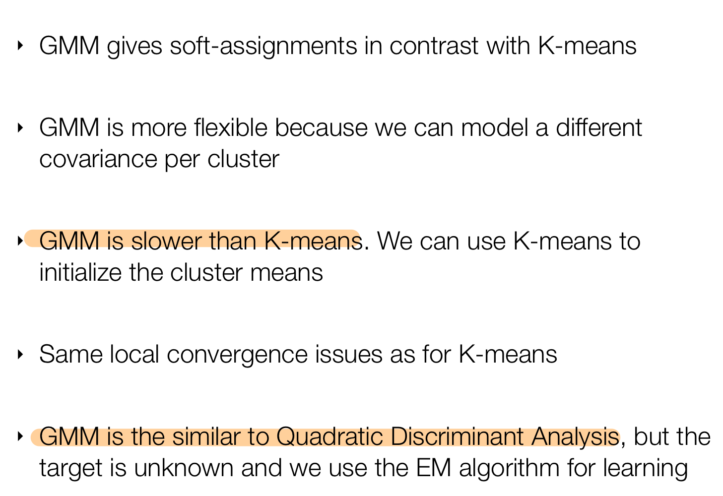
- We need more initializations in GMM because of different parameters so the trick its to do it with k-means
- Same as k-means we cannot expect to find the best solution so the global minimum for the parameters because the problem its not convex. That means the final solution depends on how you initializes the model parameters
- The last point refers that GMM is for unsupervised learning so you compute things with the latent variable whereas in QDA its for supervised learning.